The absurd efficiency of transfer learning for computer vision and machine learning

Introduction

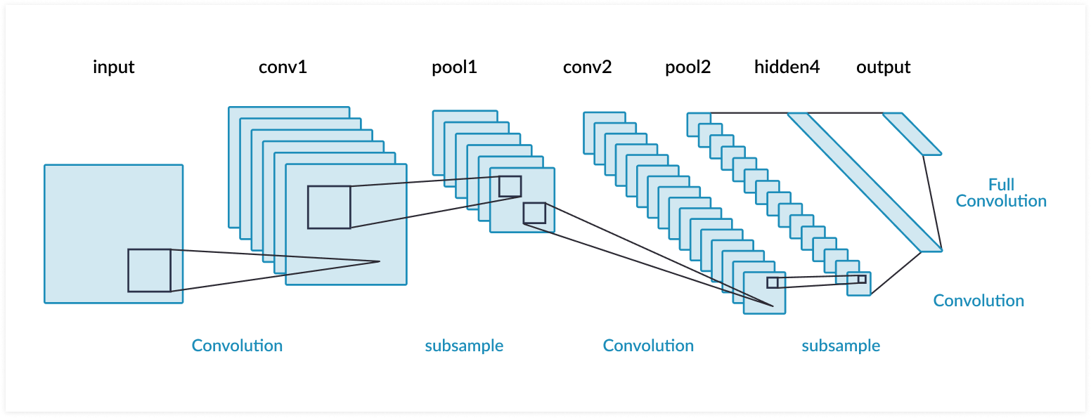
Transfer learning is a computer vision technique to quickly classify images, and is particularly powerful when you don’t have a lot of training data. The idea is to take a pre-trained neural network and then fine-tune it for a specific task, that is, transfer the knowledge learned from a large dataset to the task at hand using a smaller dataset. I used a pre-trained convolutional neural network (CNN) model that was trained on ImageNet, which consists of over 14 million labeled images. This large dataset enables the model to learn high-level abstractions for image features such as shapes, objects, and textures. Deep neural networks, and CNNs in particular, learn hierarchical feature representations, meaning that the specificity and complexity of the learned features increases as a function of layer number. So the first couple layers might learn basic things like edges, shapes, and gradients while the deeper layers recognize things like eyeballs and rollerskates. Using a pre-trained model that already knows about both low-level and high-level abstractions is incredibly powerful.

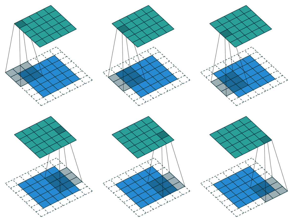
So how does computer vision work, and what’s a convolution? A convolution operation takes an initial tensor (or image) as an input, and a filter traverses the entire image. At each step of the filter traversal, the input sub-elements (where the filter overlaps the input) is multiplied element-wise by the filter itself, and the output is the sum of the products. After a convolution layer, CNNs often use pooling layers to reduce the dimensionality of the data to streamline computation. To perform classification, the output of a pooling layer is flattened (turning a 2D array into a vector) and one or more fully connected layers is used to make the categorical prediction.

CNN schematic — *Figure 2 - Example of a 7 layer CNN. In practice, CNNs can have 50 layers or more.*

Vanishing Gradients and Residual Networks

Deep CNNs with multiple layers can be tricky to train due to the problem of vanishing gradients. Recall that in a CNN, the filter weights are learned using backpropagation. This process consist of minimizing the prediction error by adjusting network weights using the gradient of the loss function. Calculating the gradient is just a matter of applying the chain rule you learned in basic calculus. The problem is that when the network is too deep, the chain rule becomes very long, and multiplying small numbers again and again will quickly make the product shrink to zero. When that happens, the weights cannot update their values during training and the network error remains large. In other words, the network doesn’t learn.

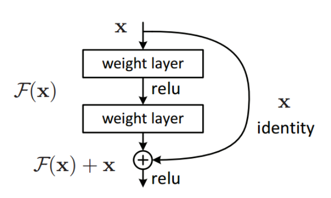
Residual block — *Figure 3 - A building block for Residual learning.*

Residual Networks (ResNets) are a modified version of CNNs and solve the problem of vanishing gradients using a residual architecture, which consist of skip connections, or identity mappings, that are added to a layer’s output. Therefore the output of a residual block consists of the sum of two terms: the layer’s normal nonlinear activation, and the original input to the residual block (Figure 3). By doing this, vanishing gradients are avoided because the gradients can flow directly through the skip connections backwards from later layers to initial filters. Variants of this idea include networks with all layers connected to each other (DenseNet), and networks that use forget gates to control how much information flows to the next time step (Long Short-Term Memory, or LSTM).

Training images — Figure 4 - Random selection of training data and the image labels (Lake, Ocean, Surfing, Tubes). Surprisingly, even with a relatively small amount of training data, transfer learning can properly classify these types of images with high accuracy.

Procedure

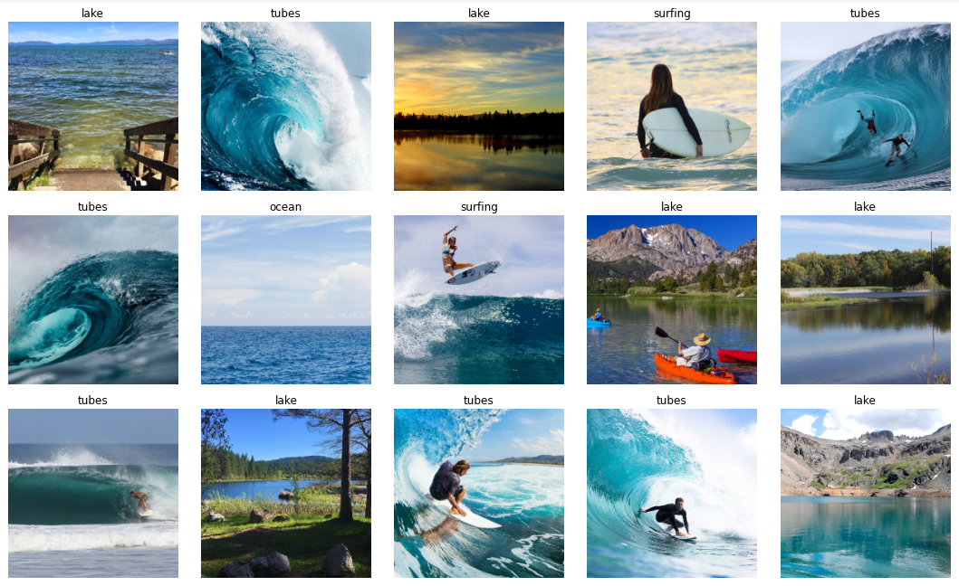
I used about 200 images for training and labeled them according to following categories: Lake, Ocean, Surfing, Tubes, (only 50 or so images in each category). 80 images were used for validation, and these were different images than the training dataset, of course. I chose these images because

1) Waves are beautiful and I love riding them, and 2) I wanted to make the image classification task challenging by using water in all the images.

A pre-trained ResNet model with 34 layers was used (over 21 million model parameters). The trick to transfer learning is to initially restrict training on the new set of data to the last group of layers in the network. After this initial training, the weights for the entire network can be updated, if needed, but you should use different learning rates for different layers of the network. The reason is that the weights in the lowest layers should not be changed much, as these layers have already been pre-trained to detect basic features such as edges and outlines using ImageNet. During training on our set of data, the last group of layers in the network gets a higher learning rate so that the high level features that are specific to our dataset, such as the circular shape of barrelling waves and the various body positions of surfers, are learned.

In addition to transfer learning, I used the one cycle learning rate policy, meaning that the learning rate was increased initially, and then decreased. The purpose of doing this is to prevent the network from getting stuck in local minima of the loss function.

Results

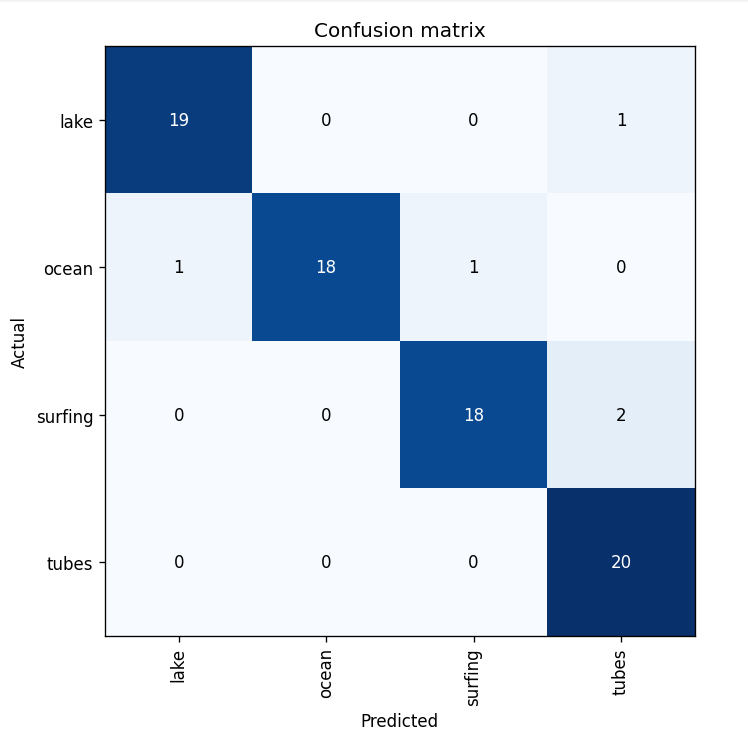
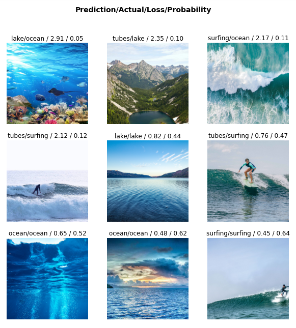
The confusion matrix in Figure 5 summarizes the performance of the image classification ResNet model on the validation dataset. The table shows the number images that lie in each matrix cell of actual versus predicted categories. A model with perfect accuracy would only have finite numbers along the diagonal and zeros everywhere else. Keep in mind the model never saw these validation images during training, so the performance is actually quite amazing considering how small the training data set was. Using just a handful of training passes through the data (10x one cycles), the model accuracy for the validation images is over 93% (only 5 incorrectly classified images out of 80). Figure 6 shows a random sample of correctly classified images, as well as the incorrect predictions. It’s not too surprising that the model classifies some of these images incorrectly because similar images they were not common or were non-existent in the training dataset (such as the image of the aerial shot shown in the upper right corner of Figure 6). In addition, the model provides information about whether or not you should trust the prediction, because the last layer of the neural network outputs a probability (softmax activation function). In general, the probabilities are less than 0.5 for the incorrect predictions, showing that you could filter the output if you needed a high true positive rate (although your false negative rate would increase).

Just as with computer vision, natural language processing (NLP) models can also benefit from transfer learning. Here is a paper demonstrating this technique for common NLP tasks such as sentiment analysis, question classification, and question answering. And here is a paper that takes this concept to the next level and tests few-shot learning with the GPT-3 language model. So hopefully I’ve convinced you that using a pre-trained model is extremely powerful, and perhaps you learned something about the algorthims behind things like self-driving cars.

Predictions — Figure 6 - The predicted and actual categories of some of the validation images. The 5 incorrectly labeled images are shown here, along with some of the correctly labeled images. Apparently the arc-shaped outline of the lake was interpreted as a barrelling wave (i.e., Tube) in the 2^nd image. Also, the network incorrectly thought that two images of mushy waves were actually tubes. However, overall the network is extremely accurate!

Credits

Images were pulled from Google Images, and I used the fastai library to train the ResNets for this project.